Examples - Time series
ADAMS' efficient token-passing architecture makes it ideal to handle streams of data. It is also very easy to extend. In these examples, we introduce new actors for several signal analysis techniques, and show how we can quickly build and test workflows to analyse time series data.
Note: the videos should only be considered educational, as some of the concepts in ADAMS have changed over time. E.g., global actors are now called callable, since they can appear in different scopes within the flow. Also, SingleFileSupplier and MultiFileSupplier got merged into the FileSupplier actor.
Convolution - Finding the signal in the noise
Sensor data is often noisy and complex. Here, we introduce an actor for convolution, an operation that transforms the data into something more useful.
Smoothing
First, we convolute the signal with a Gaussian response function (or kernel) to obtain a much cleaner signal.
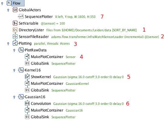
Retrieve data files from the given folder. Emits the files as tokens.
Load and interpret the files and emit [timestamp,sensorvalue] tokens for every new timestamp.
Branch actor: each token is sent to three subflows for further processing.
This branch simply plots the data. Timestamp and sensor value are mapped straight to an X and Y coordinate, [X:timestamp,Y:sensorvalue], then sent to the plotter.
Visualize the used kernel (here, a Gaussian kernel). Emits values to plot the kernel, centered on the received timestamp.
Convolute the received data with the kernel. The agent buffers the last N tokens (N=kernel width), and emits the convoluted data points.
Global plotter for all data. Receives tokens sent to all GlobalSink actors linked to it.
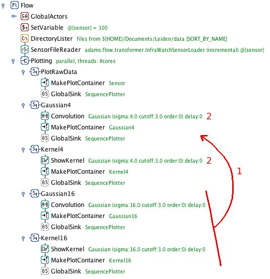
Smoothing at different levels
Changing the width of the kernel allows us to focus on events occurring on different time scales. Simply copy-paste the last two branches and change the kernel widths.
Scale-space composition
Convoluting the same signal with a whole range of different kernel widths creates a so-called scale space, a space of signals sensitive to events at different time scales.
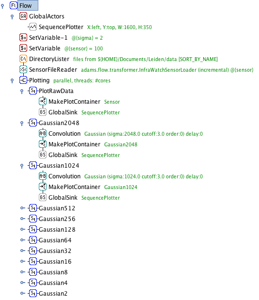
Copy-paste the convolution branches
Increase the kernel width. Here, we double it each time
Scale-space decomposition
Decomposition of a sensor signal into components displaying events occurring on different time scales. Detecting transient events when these events occur on different timescales in data prone to baseline shifts can be very tricky. Through scale-space decomposition, we decompose the raw signal into its natural components, and use those to detect events. This is done by taking the scale space and establishing 'regions' of the scale space where events of a certain time scale take place. Each region will be represented by a component, calculated by substracting the convolutions at either end of the region. The latter is also known as a 'difference of Gaussians' filter, or band-pass filter. The sum of the components recreates the original signal.
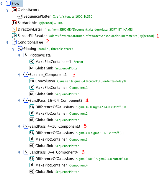
Sensor data is read and split into individual tokens as before
The data is subsampled: only every 100th token is passed on
The baseline of the data is created through convolution with a large Gaussian, only sensitive to large-scale events
The first band-pass filter is applied. It takes the difference of the Gaussians of width 64 and 16. The result is sent to the plotter
Second band-pass filter, for signals in the range sigma=[4,16]
Third band-pass filter, for signals in the range sigma=[0,4]
Segmentation of time series data
A time series can be approximated by a piecewise linear function. This will result in a time series that is significantly smaller in size (disk space), and thus easier to store and process.
Segmentation through convolution
One way of approximating the signal is to begin a new line segment if the signal changes it's slope drastically. These points can be found by taking the 1st, 2nd, 3rd,... order derivative of the signal and start a new line segment for every zero-crossing of these derivatives. Instead of first calculating the convolution of a signal and then taking its derivative, we can achieve the same result by convoluting the signal with the derivative of the kernel used for convolution! Thus, we take the 1st, 2nd, 3rd,... order derivative of the Gaussian kernel, do their convolutions, and start a new line segment at any zero-crossings.
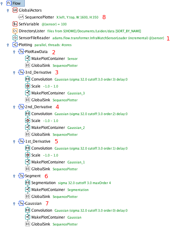
Load and split the data into tokens as before
Plot the raw sensor data
Compute the third order derivative of the convolution and normalize it between -1 and 1 (for nicer plotting)
Compute the second order derivative of the convolution and normalize it between -1 and 1
Compute the first order derivative of the convolution and normalize it between -1 and 1
The segmentation agent does the same as the above three branches, but only lets through a token (unaltered) if one of the derivates crosses zero
Compute and plot the convolution with the base Gaussion kernel
The plotter collects and plots all received tokens
Discrete Fourier Transform of sensor data
Applying DFT
Applying discrete fourier transformation to the sensor data and displaying the frequency domain.
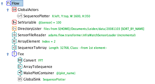
Select the FFT Conversion in the Convert actor.